
The Real Symptom
Your GPU bill is climbing. Your utilization dashboards tell a different story: 15% average, maybe 30% during peak hours. You’re paying for expensive capacity that spends most of its time waiting—on underfilled batches, slow CPU pipelines, or serving overhead.
This is primarily a systems design problem. Buying more GPUs—or upgrading to the latest generation—doesn’t fix it. It amplifies it. Burn rate increases, capacity planning becomes guesswork, and your team spends more time managing infrastructure than improving models.
In many production AI systems, a large share of GPU capacity goes unused—not because the hardware is wrong, but because the surrounding system (batching, data pipelines, scheduling, memory behavior) was never designed for sustained utilization under real traffic variance.
Here’s a practical way to address it.
The Four Root Causes of Poor GPU Utilization
Before changing anything, isolate where the idle time comes from. Most cases fall into four buckets.
Underfilled batches
GPUs are efficient when they run large parallel workloads. A batch size of 1 wastes most of that potential. In production, traffic is uneven—bursts followed by silence—and request shapes vary (sequence length, image size, etc.). Without batching strategies, your GPU processes small jobs while it could process dozens.
How you notice it: low throughput, small batch sizes, high kernel launch overhead, and a utilization pattern that spikes briefly then drops.
CPU and data pipeline bottlenecks
The GPU can’t process what it hasn’t received. Tokenization, image preprocessing, data loading from disk or network—these live on the CPU. If the pipeline can’t feed the GPU consistently, utilization collapses regardless of how powerful the accelerator is.
How you notice it: high CPU time per request, high I/O wait, or queueing happening before the GPU stage while the GPU sits underutilized.
Inefficient model execution
Some inefficiencies are self-inflicted: running FP32 when FP16/BF16 suffices, unoptimized kernels, poor memory locality, or KV cache fragmentation for LLM serving. These don’t always produce obvious errors—they quietly reduce effective throughput.
How you notice it: utilization might look “okay,” but tokens/s (or images/s) is low for the hardware, memory bandwidth is saturated, or you see frequent allocator churn/OOM retries.
Scheduling and serving overhead
Context switching between models, cold starts, suboptimal routing, and small requests that don’t amortize launch overhead add up. Even with decent batching and pipelines, a serving layer that routes poorly or spins instances inefficiently will create idle time.
How you notice it: rising queue wait time, p95 latency drift, frequent cold-start spikes, and variability that correlates with deployment or routing changes.
A Practical Optimization Framework
Metrics That Matter
You can’t optimize what you don’t measure. Focus on a small set of signals that tell you where time and cost are going:
GPU SM occupancy (how busy the GPU actually is)
Memory bandwidth utilization (are you compute-bound or memory-bound?)
Throughput (tokens/s or images/s—define your unit of work)
Queue wait time (how long requests wait before hitting the GPU)
p95 latency (tail latency drives user experience)
Cost per unit of work (e.g., $/1,000 tokens or $/request)
Cache hit rate (KV/embedding/response cache where applicable)
The key is correlation: utilization alone can drop when traffic drops. You need to see how utilization relates to throughput, queueing, and tail latency.
The Trade-off Triangle
Every optimization involves trade-offs across throughput, latency, and cost/quality.
Larger batches improve throughput and cost efficiency, but can increase p95 latency.
Quantization reduces cost and increases throughput, but may affect quality and requires careful validation.
Aggressive caching improves performance, but introduces correctness, privacy, and invalidation concerns.
There’s no free lunch—only deliberate choices aligned with your product requirements and SLOs.
High-Leverage Techniques
Dynamic batching
Accumulate requests over a short window (typically 5–50ms) before dispatching to the GPU. This fills batches without adding unacceptable latency. Tune the window against your p95 latency SLO: tighter for real-time apps, longer for batch workloads.
Trade-offs / failure modes: batching can worsen tail latency if the window is too large, and mixed request shapes can cause OOM if you batch without bucketing by size/length.
Request coalescing and queue management
Not all requests are equal. Group similar requests (same model, similar sequence length/image size) to maximize batch efficiency. Use priority queues so latency-sensitive traffic isn’t blocked by bulk jobs.
Trade-offs / failure modes: more complexity and routing logic; requires workload characterization and guardrails to prevent starvation.
Caching strategies
For LLMs, KV cache reuse across requests with shared prefixes can remove redundant computation. Embedding caches help retrieval-heavy systems. Response caches can work when exact queries repeat.
Trade-offs / failure modes: memory overhead; correctness and invalidation; and in multi-tenant systems you must ensure cache keys enforce isolation to avoid data leakage.
Mixed precision and quantization
FP16 or BF16 often matches FP32 quality while increasing throughput and reducing memory. INT8/INT4 quantization can push further—but needs calibration and robust evaluation.
Trade-offs / failure modes: quality regressions can be subtle; require an evaluation harness (golden set + regression checks) and release gates tied to acceptance criteria.
Model serving optimizations
Use optimized inference engines where appropriate (operation fusion, better memory access patterns). Warm up models to avoid cold-start latency. Use pinned memory (where supported) to reduce transfer overhead.
Trade-offs / failure modes: more operational complexity; some optimizations are model-specific and may increase debugging difficulty without good observability.
Data pipeline acceleration
Pin data-loading processes to specific CPU cores. Use async prefetching so data is ready before the GPU needs it. Avoid Python bottlenecks in hot paths—offload to compiled code or use multiprocessing where it makes sense.
Trade-offs / failure modes: more moving parts; can backfire if you optimize the wrong layer without profiling.
Right-sizing and intelligent autoscaling
Scale based on queue depth, throughput, or tokens/s—not CPU utilization. GPU workloads don’t correlate well with CPU metrics. Set minimum replicas to reduce cold starts and maximums to control cost.
Trade-offs / failure modes: requires custom metrics and careful thresholds; risk of under-provisioning during spikes if you scale too slowly.
Observability (so you don’t optimize blind)
Monitoring GPU utilization alone is not enough. Utilization can drop simply because traffic drops. The signals that matter are system-level: queue wait time, throughput, batch size distribution, and tail latency.
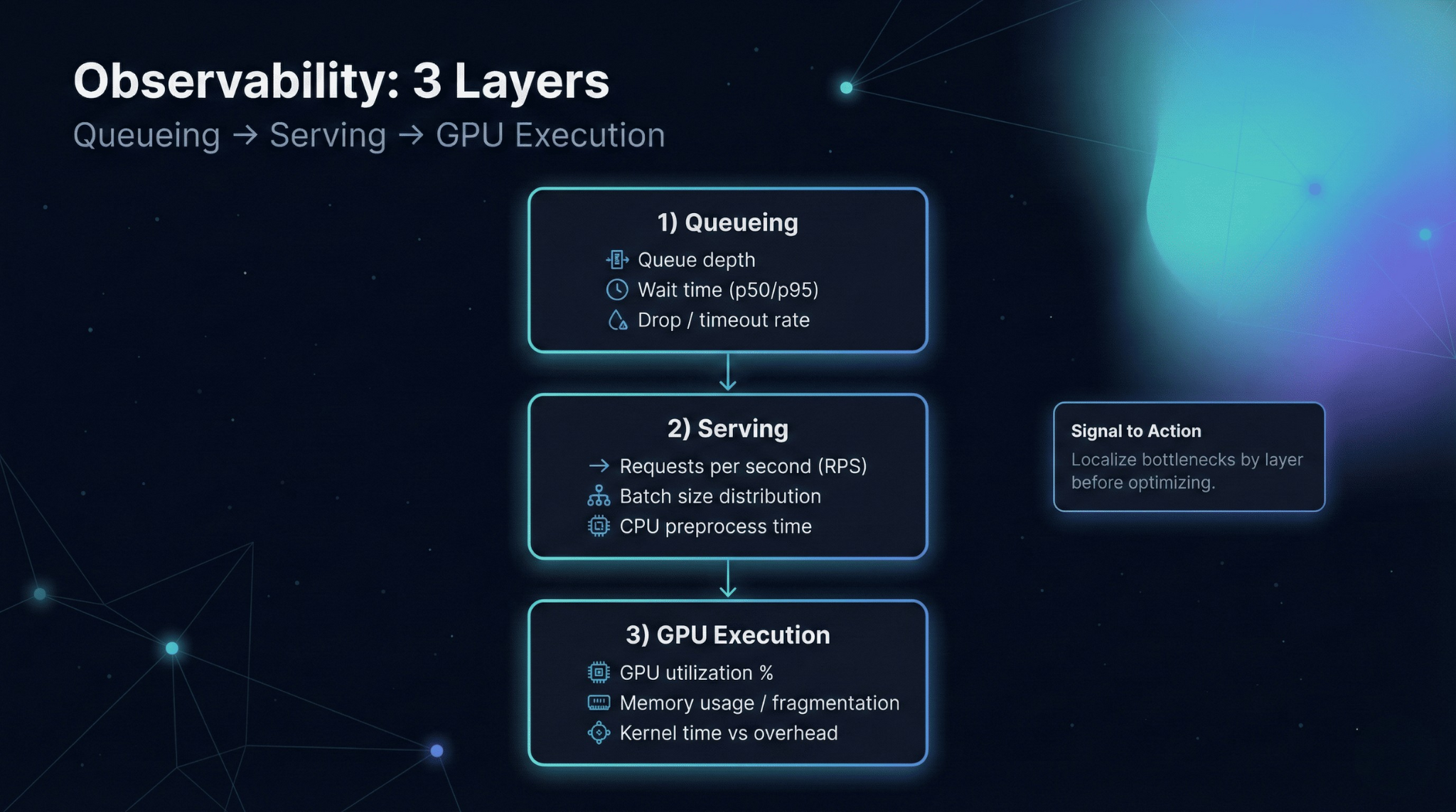
Instrument at three layers:
Queueing: queue depth and wait time (is the GPU starved or overloaded?)
Serving: batch sizes, request shape buckets, cache hit rates (are you doing efficient work per batch?)
GPU execution: SM occupancy, memory bandwidth, OOM/retry rates (are kernels and memory behaving?)
Alert on changes that correlate with user impact: rising queue wait time, throughput regression, or p95 drift—then use GPU metrics to localize the cause.
Production Checklist (Release Gate)
Before and after any optimization, verify the minimum set below:
Capture baseline: utilization, throughput, p95 latency, queue wait time, cost/unit
Validate quality: evaluation set unchanged + output validity checks
Verify stability: error/OOM/retry rates not worse
Test peak load: p95 and queue wait time within SLO
Confirm rollout: canary/shadow + rollback path works
Update dashboards: queue + serving + GPU layers (not just utilization)
Mini Scenario
Before: A text generation service running on 8 GPUs. Average utilization: 18%. Cost: $0.012 per 1,000 tokens. p95 latency: 420ms.
Changes applied: Implemented dynamic batching with a 25ms window. Enabled KV cache reuse for common prefixes. Switched to BF16 precision after validation.
After (illustrative): Utilization increased to 62%. Cost dropped to $0.004 per 1,000 tokens. p95 latency improved to 380ms. GPU count reduced to 4 with headroom for growth.
The point isn’t the exact numbers—it’s the pattern: batching + cache reuse + precision choices compound when you measure, isolate bottlenecks, and validate with guardrails.
The Principle
GPU optimization is a systems problem. No single technique delivers transformational results in isolation. The gains come from systematic measurement, bottleneck isolation, and deliberate trade-offs aligned with product requirements.
Start with observability. Identify your dominant constraint—batching, data pipeline, model execution, or scheduling. Apply targeted fixes, one at a time. Validate against latency SLOs and quality gates. Keep rollout and rollback disciplined.
The goal is not 100% utilization. The goal is predictable, cost-efficient performance that scales with your business—and remains operable under real traffic, real failures, and real on-call conditions.